Projects ECG (Electrocardiogram) Monitoring

QRS complex J point II

In the section of QRS complex J point I, I covered cases where the S wave does not exist or does not appear clearly. This time, we look at a case where the S wave is evident.

Although there are quite a variety of cases and they are complex, I introduce them here by introducing a boundary condition.

Case 1.

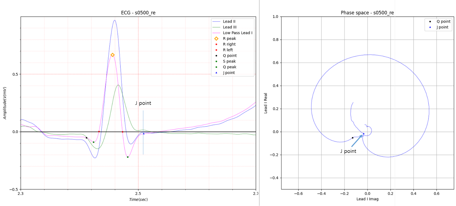
Fig.1

Fig.1 is an electrocardiogram in the absence of cardiopathy.

This example is a case where there is no peak after S peak.

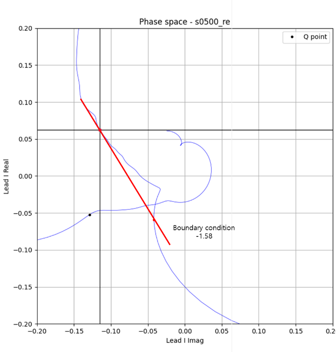
Fig.2 Boundary condition

Boundary condition is shown in Fig.2.

This red line is a tangent line obtained from the peak of the S wave in the X-axis negative direction and the peak of the T wave in the X-axis negative direction to the peak of the S wave in the X-axis direction.

J point is the first imaginary peak.

This was introduced in the ecg_patent3.

Case 2.

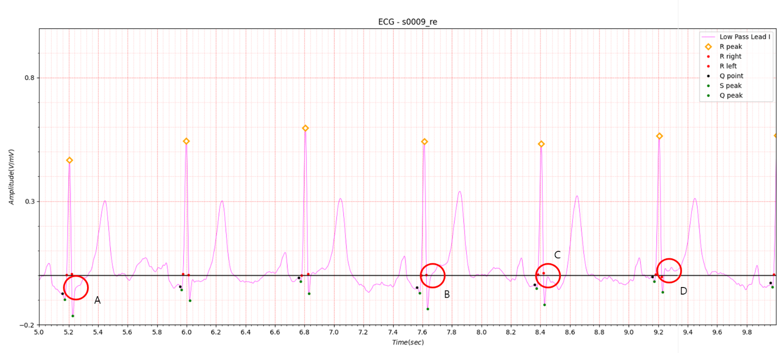
Fig.3

Case 2 is the case that led to the introduction of the boundary condition and made me feel that my idea that electrocardiogram diagnosis could be sufficiently performed with a single lead was just a dream.

Fig.3 shows the complexity of case 2.
I will introduce each boundary condition for the red circles in Fig.3 and show that ECG diagnosis is possible with a single lead by applying this boundary condition.

Fig.2 shows the S wave bending sharply in the direction toward the T wave, and in this case, the starting position of the boundary condition leaves a peak in the negative direction on the X-axis. However, if it is bent gently, there is no peak in the negative direction on the X-axis.

At Fig.4, the negative peak in the X-axis direction does not exist in the S wave. In this case, the starting position of the boundary condition becomes the Imaginary peak.

s009_re The electrocardiogram has about 10 boundary conditions. This ECG data shows quite complex aspects, so I briefly introduce five cases.

I will distinguish various types of cases using the angle of the boundary condition line.

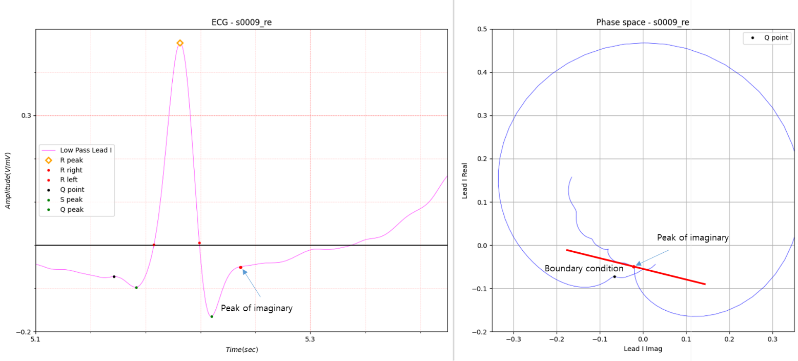
Fig.4 Part A of Fig.2

In Figure 4, since the starting point of the boundary condition is the Imaginary Peak, the straight line connecting the Imaginary Peak and the first peak is determined as the boundary condition Line.

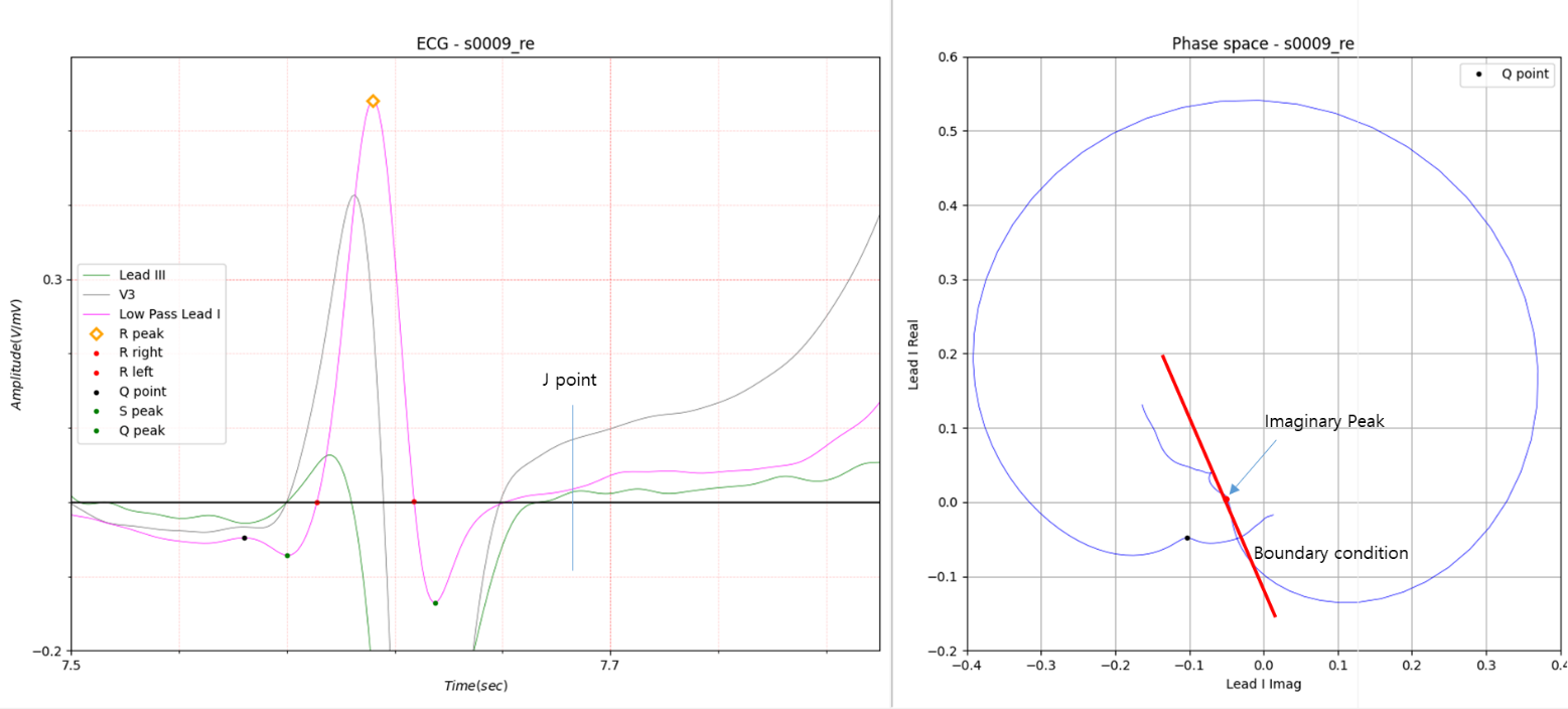
Fig.5 Part B of Fig.2

In Figure 5, since the starting point of the boundary condition is the Imaginary Peak, the straight line connecting the Imaginary Peak and the first peak is determined as the boundary condition Line.

The difference from Figure 4 lies in the slope of the boundary condition line.

In Figure 4, the slope of the boundary condition line is less than 1, and in Figure 5, it is greater than 1.

As shown in Figure 4, if the slope of the boundary condition line is less than 1, the J point is an imaginary peak that exists in the middle of the first and second peaks.

As shown in Figure 5, if the slope of the boundary condition line is greater than 1, the J point is an imaginary peak that exists just before the first peak.

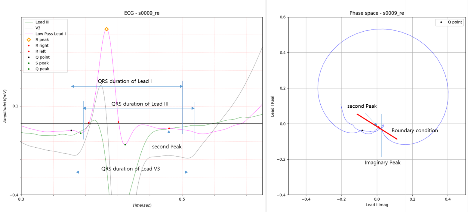
Fig.6 Part C of Fig.2

In both the previous two cases, the first peak was used as the boundary condition.

Based on the first peak in Figure 6, the slope of the boundary condition line is positive and close to vertical. In this case, if a second peak exists, the second peak is included in the boundary condition.

After passing the second peak, there is a downward peak (valley) below the boundary condition line. In this case, the first imaginary peak after the second peak is the J point.

To verify whether the J point determined in this way was correct, Lead III and Lead V3 were compared. The three QRS durations are perfectly consistent.

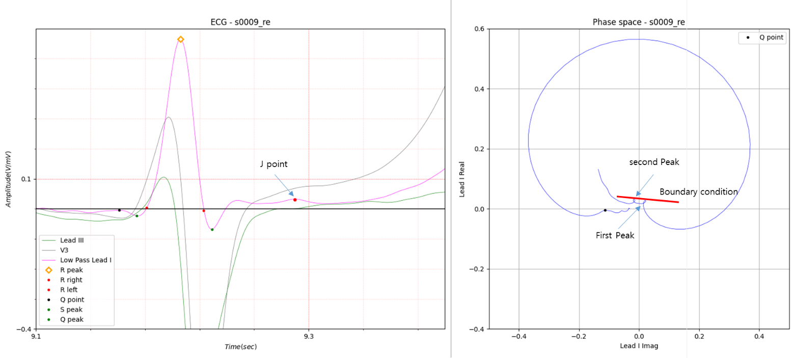
Fig.7 Part D of Fig.2

Figure 7 is basically similar to Figure 6. However, both peaks in Figure 7 have small rings. As shown in Case 3, large peaks form a large circle and small peaks form a ring shape. The tiny peaks, which are not easily visible to the eye, have a notch shape.

The two peaks have slopes close to horizontal. In this case, J point is the second peak.

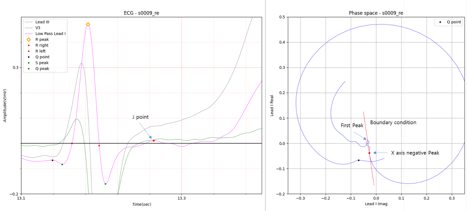
Fig.8

In Fig. 8, the first peak has a notch shape and a positive slope that is close to vertical. Therefore, the second peak is set as the boundary condition. The slope of the boundary condition line is negative and close to vertical. In this case, the second peak is set as J point.

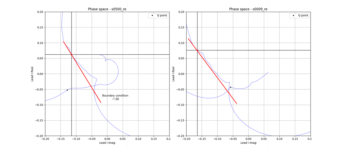
Fig.9 similar boundary condition

In Fig. 8, the first peak has a notch shape and a positive slope that is close to vertical.

In Figure 9, Case 1 and Case 2 have similar the slope of the boundary condition line. The difference is that case 1 has no noticeable peak and case 2 has a downward peak. In this way, a method of obtaining the J point was introduced by introducing various boundary conditions.

The QRS duration results for Case 2 obtained in this way are shown below. This result shows a fairly stable result considering the ECG data, which has a fairly complex shape.

39 [126 124 129 124 127 127 125 126 122 120 129 121 131 133 123 127 122 128 120 132 129 135 125 132 125 121 135 120 127 134 136 136 131 126 127 130 130 134 135]

Max: 136 Min: 120 average: 127.79 standard deviation: 4.79

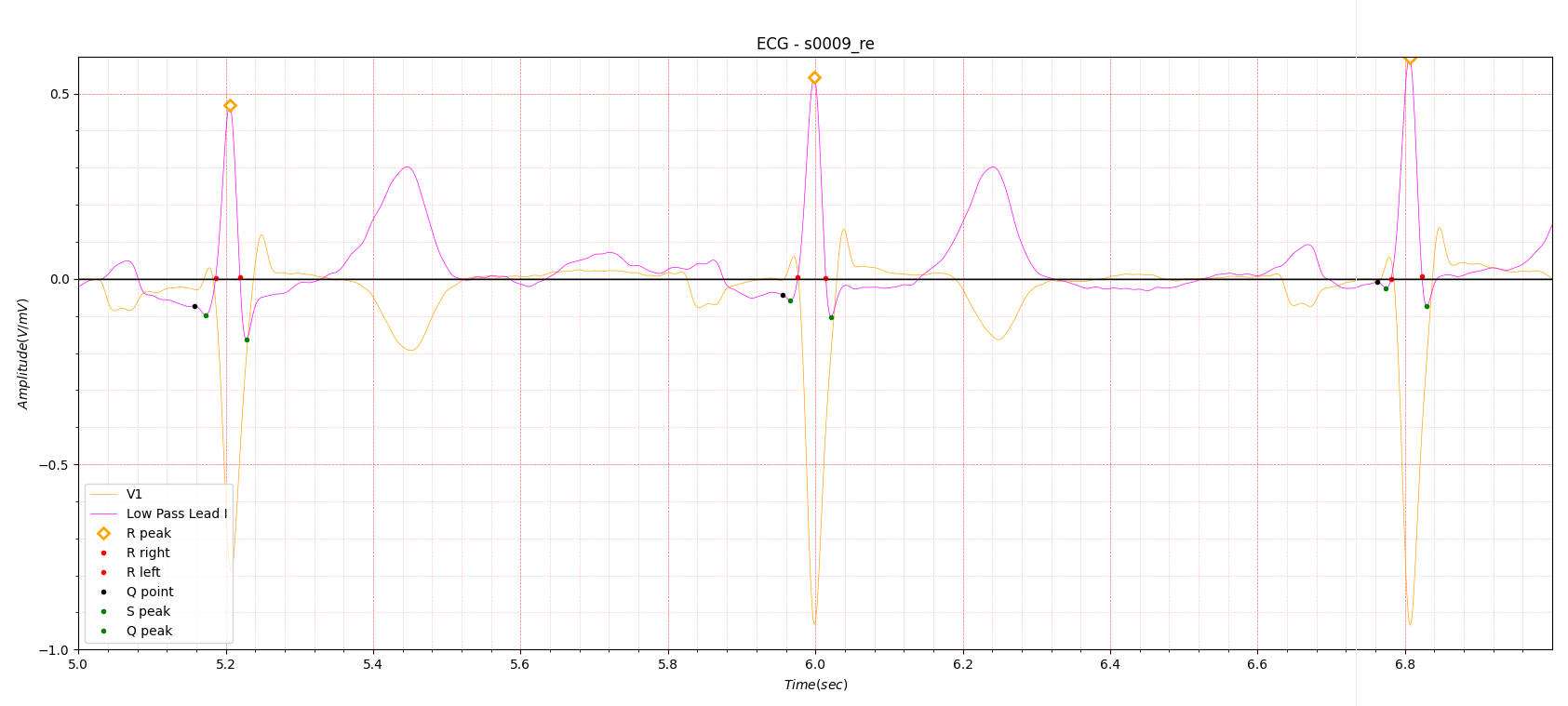
Fig.10

Figure 10 shows lead I and lead V1 together. Lead v1 is a typical Right Bundle Branch Block in the shape of rabbit ears.

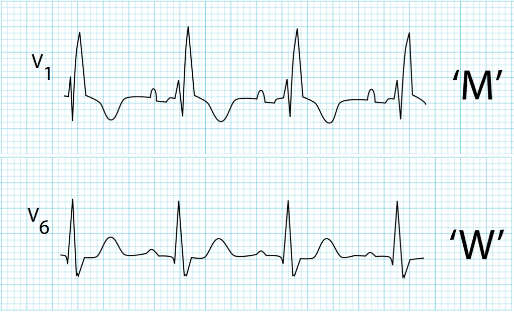
Fig.11 Right Bundle Branch Block

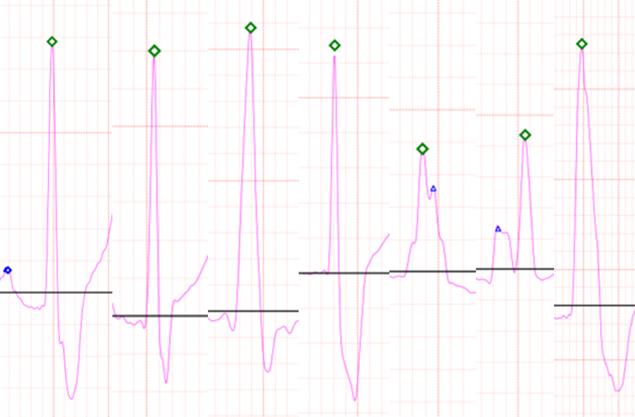
Fig.12 Various type of Bundle branch block

Figure 12 shows various types of bundle branch blocks.

Case 2 shows that cardiopathy, which is difficult to find in a single lead using general methods, can be found. Although the standard for bundle branch block is a QRS duration exceeding 120, it often exceeds 120 in cases of myocardial infarction.

The distinction from myocardial infarction will be introduced gradually in the future.

Case 3.

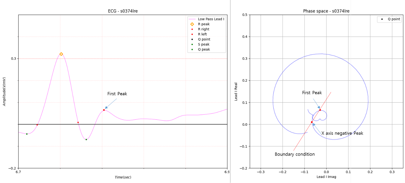
Fig.13

Figure 13 shows a case where a large peak exists at the end of the S wave. As introduced earlier, the large peak forms a circle. It is difficult to define large peaks using general methods. This means that it is difficult to define what a large peak is based on prominence. When the slope of the boundary condition line approaches 1, the J point is the first downward peak (valley) passing through the peak.

Case 4.

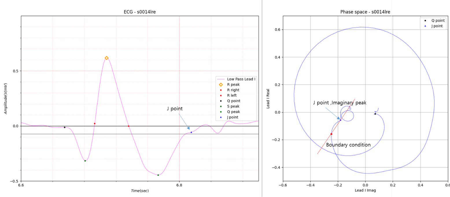
Fig.14

Figure 14 resembles the case in Figure 13. However, there is an imaginary peak before the first peak. The slope of the boundary condition lined has a value close to 1 in the positive direction. In this case, the location of the J point is the Imaginary peak.